

We interviewed Hani Habra, one of the co-authors of the software tool Binner: a desktop application for annotating isotopes, adducts, and in-source fragments in untargeted metabolomics data produced by electrospray ionization liquid chromatography mass spectrometry (ESI-LC/MS).
Tools like Binner drastically reduce the complexity of untargeted metabolomics datasets. Without them, it would be much harder to glean meaningful insights from the measurements because the noise tends to drown out the signal we’re searching for.
How one metabolite produces multiple signals
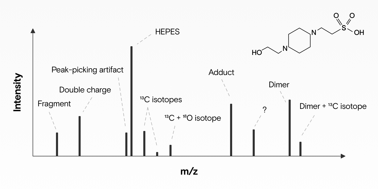
If we analyze a biological sample (e.g., blood) with an electrospray ionization mass spectrometer, then a single metabolite (e.g., a small molecule in the blood) produces not just one signal, but many. There are four reasons for this:
- Isotopes: Several isotopic versions (isotopologues) of a molecule are usually present. This means it’s the same molecule, but one or more of its atoms has a different number of neutrons. For example: ~1.1% of all carbon atoms on Earth have 7 neutrons rather than 6. If our molecule has 1 carbon atom, then we’ll likely also observe a second mass peak with ~1 dalton higher mass (M+1) and a roughly 99% lower abundance in our mass spectrum.
- Adducts: New molecules form when two or more molecules combine. A portion of the molecules we want to measure also combine with others to form new molecules (adducts). What adducts can form depends on many things: How you prepare your sample (e.g., which solvent you use: acetone or formic acid), how samples were stored, and whether you run your machine in positive or negative ion mode. A simple and common example is adducts that are formed when sodium atom (Na) or proton (H+) is added.
- Fragments: When molecules are ionized in a mass spectrometer, some ions become energetically unstable and may subsequently break up. Usually one of the resulting fragments has a neutral charge and is therefore undetectable, while other - now smaller - charged fragment ions remain. These fragments show up as additional signals. If we know what neutral losses to expect, then we can group these fragments together with the original molecule.
- Multimers: Complexes may form between two or more metabolite monomers, in addition to charged species, generating an m/z value that is typically around 2-3 times that of the individual metabolite.
So what was originally just one molecule turns into many measurements – and this is a significant obstacle to any analysis.
Why splitting signals makes downstream analysis more difficult
So one molecule produces not just one but many signals. This makes it hard to determine precisely how much of one particular molecule was in the sample that we’re measuring.
This presents several important problems:
- Patterns are harder to spot: If you’re looking for a difference between two groups of patients (e.g., those who have a disease and those who don’t), finding these differences will be much harder if the information is fragmented over many signals. The pattern you’re looking for might disappear altogether.
- Multiple comparisons create chance patterns: The more signals we search through, the more likely we are to find a seemingly nice pattern that was actually produced by chance (see multiple comparisons problem). The more distinct compounds we have, the worse this problem gets.
- Features are redundant: Signals originating from the same source ion are probably highly correlated. So when the number of interesting-looking features is multiplied, our downstream analysis becomes more cumbersome and redundant.
- Biological correlations are hidden: The correlations between redundant features make it harder to find correlated metabolites - making it harder to learn more about the involved biological pathways.
- Signals are misidentified: The more signals we have the easier it is to make mistakes. We might connect signals that don’t belong together, or we might identify a signal as its own metabolite when it’s actually derived from another.
All of this makes it much harder for us to find the meaningful insights we’re after. What’s more, we might even find insights that are simply false.
That’s why it’s very important to correctly identify as many of the derivative features as we can and group them together. The process of determining how signals belong together is called annotation, because we annotate signals with descriptions of how they develop from a precursor ion. This is what Binner helps us to do better.
How feature annotations worked before Binner
Binner isn’t the first tool to help annotate features. The R-tool CAMERA has been popular for almost 10 years, and there are many others.
Before Binner, there were five main techniques that feature annotation tools used to determine which signals belong together:
- Retention time grouping/ thresholding: The retention time of associated features has to be very similar – i.e., the features should co-elute. Usually the tool sets a certain tolerance for retention time groups, and if there’s a gap between two signals longer than this setting, then the tool creates a new group of features.
- Correlation: Features originating from the same metabolite probably correlate. So you can use all the measurements in your batch to calculate correlations between features, and those with higher pairwise correlation are more likely to belong together.
- Clustering: After binning features by retention time and calculating pairwise correlations, tools often use one of several clustering algorithms to group features together based on a similarity metric (e.g., correlation).
- Chromatographic peak-shape similarity: Adducts and fragments should have a similar peak-shape, since they originate from the same metabolite – which exits the LC column in a specific abundance curve.
- Relative adduct frequency: Based on prior knowledge and the observed frequencies of different adducts in similar datasets, we can make assumptions about which fragments are more plausible than others.
Binner combines several of these existing techniques and then goes even further, offering helpful visualizations.
How Binner annotates features
Like the other tools, Binner – the tool Hani Habra co-developed – automatically groups features that come from the same metabolite.
It aims to reduce the features in your dataset significantly – leaving as many 1–1 relationships between features in the dataset and real-world compounds (molecules) as possible.
Here’s a step-by-step overview of how Binner works:
- Binning retention time: Binner groups features based on differences in elution or retention time into self-contained units called bins.
- Calculating correlations: Next it calculates the pairwise correlation based on abundance values for each feature in a bin.
- Detecting isotopes: It finds and groups C13 isotope versions of features, assuming isotopes must decrease in abundance as their mass increases (since C13 is naturally less abundant than C12).
- Hierarchical clustering: Next, Binner clusters features using their correlation vectors and optimizes the number of clusters to minimize the average per-feature silhouette value.
- Centering the most abundant feature: It uses the most abundant feature as the basis for the following adduct hypotheses.
- Testing hypotheses to explain mass differences: Binner then tests the most frequent ions – including the user-supplied list of adducts and neutral losses/gains – to explain mass differences. Then it keeps the hypothesis that annotates the maximum number of features in a particular group.
- Repeating: Finally, Binner tries to annotate the rest of the ions, starting with the next most abundant unannotated ion.
How the annotation file guides Binner’s assumptions
As with some other tools, you provide Binner with an annotation file containing the charge carries, neutral gains, and neutral losses you expect to see in your dataset.
Unlike some other tools, Binner doesn’t restrict itself to the exact adduct formulation you provide. It also allows for adduct combinations of anything that’s defined in the annotation file. So if you specify a charge carrier of Na (22.982) and a neutral gain of Na - H + NaCOOH (89.97), then it’s conceivable that Binner will annotate features as "M+Na + Na - H + NaCOOH" (which can be simplified to M+2Na-H+NaCOOH).
But Binner doesn't stop there – it does more than just automated annotations.
Making annotations transparent
Binner also provides visual explanations for its annotations. This helps you to understand why features have been grouped and annotated in a particular way, which gives you confidence in the annotations.
Binner also displays information you can use to find and define new, previously unknown adducts to add to your annotation file, significantly increasing the number of features you can annotate.
Let’s have a look at how this works.
Visualizing feature correlations and annotations
For each cluster Binner finds, its shows you the
- annotation it settled on, as well as the calculations of neutral losses and adducts that lead to that annotation;
- correlations between each feature in the cluster, as both values and a heatmap.

Seeing the reasoning behind each annotation also allows you to do quick plausibility checks. For example, if you see that multiple adducts were labeled: M+COOH+NaCOOH, M+COOH+2NaCOOH, M+Cl+3NaCOOH, M+Cl+4NaCOOH, M+Cl+5NaCOOH, then because each “step” is present, you can see that even the very complex adduct M+Cl+5NaCOOH is probably a reasonable annotation.
But if “2, 3, and 4” are missing from the cluster, then a complex adduct annotation like M+Cl+5NaCOOH seems much less likely to be correct.
Binner also gives you hints to help you find complex new adducts, a process Hani calls “deep annotation.”
Deep annotation: Finding novel, complex adducts
Even after a diligent automated annotation, many features will still not be annotated.
In fact, what adducts and fragment ions can form due to in-source events is not yet fully understood. And so the existing annotation files are incomplete – they don’t include anywhere near all the adducts and neutral losses that are likely to occur.
Deep annotation helps you discover currently unknown adducts that you might want to add to your annotation file:
- Binner collects the mass differences between all the unannotated ions in the dataset.
- It counts the frequency of each mass difference and highlights the most frequent ones.
- Then it suggests which adducts might explain these common mass differences.
Seeing the most common differences not only shows you which adducts you might want to add to your annotation file, but also helps you explain how these – often complex – adducts might form. Here’s an example:
A common mass difference is 43.9639, which can be annotated as +2Na-2H; another common mass difference is 67.9877, which corresponds to +NaCOOH. Together these might explain a common but previously unknown mass difference of 111.952, which corresponds to +2Na-2H+NaCOOH. You could then add this to your annotations file.
Visualizing common mass differences can help you find novel, reasonable additions to the annotation file – which in turn helps Binner to annotate a lot more previously unannotated features.
Try Binner right away
You can download and install Binner here: https://binner.med.umich.edu/. It’s simple.
The team behind Binner
Binner was developed by William Duren and Janis Wigginton; the project was led by Dr. Maureen Kachman (Analytical Chemist and Managing Director of Metabolomics Core) and Dr. Alla Karnovsky (Associate Professor of Computational Medicine & Bioinformatics at the University of Michigan) and Hani’s PhD advisor, with ample statistical/ numerical contributions to the project from Dr. George Michailidis.
Are you optimizing your metabolomics workflow?
Our machine learning team has extensive experience in metabolomics workflows. If you’re worried about how to turn research code into robust production applications, get in touch.